In this first flood mapping example we assume that the user has the relevant data on their own local device. The data required for TU Wien flood mapping algorithm consists of \(\sigma^0\) backscatter data, the projected local incidence angle (PLIA) values of those measurements, and the harmonic parameters of a model fit on the pixel’s backscatter time series.
Note
The data can be formatted to the correct structure with the files found in the GitHub repository.
1.1 Setting-up a Python Session
We begin by loading openEO for local processing and some additional packages for transforming and viewing data.
from datetime import datetimefrom pathlib import Pathimport numpy as npfrom openeo_flood_mapper_local.view_flood_map import view_flood_mapfrom openeo.local import LocalConnectionfrom openeo.processes import ProcessBuilder, array_element, add, multiply, sin, cos, mask, exp, median
Did not load machine learning processes due to missing dependencies: Install them like this: `pip install openeo-processes-dask[implementations, ml]`
1.2 Data Sources
The paths to the local data sources define the collections to be loaded in the next steps. In the case of a local openEO instance, we do this by just supplying the paths to the files required for the analysis.
Establish the local connection by supplying path(s) to root directories of the data source(s). This results in a connection object which is a critical aspect of collection discovery on the backend by openEO, where in this instance the backend is your own machine.
openEO supplies a set of conventional and EO-specific functions (or “processes” in openEO terminology) to work with EO data. In this example, we begin by defining functions that represent the flood mapping algorithm as defined in Bauer-Marschallinger et al. (2022), and by using standard openEO functions. The flood mapping algorithm extracts the following information: 1) the expected backscattering from water bodies, and 2) the expected backscatter intensity over land pixels given historical data. Hence, this function makes use of observations along both the spatial and temporal dimensions of the datacube.
We first define the function that extracts average backscatter intensity over water bodies and we name it water_backscatter(). This functions applies so-called openEO “band math”, which are basically mathematical computations on the bands of the datacube. In this case, the band of the incidence angle (degrees) of the retrieved backscatter signal is multiplied by a factor consisting of the slope plus an intercept from a linear model. This linear model describes the relationship between incidence angle and backscattering over water globally. Applying this linear model results in expected water back scattering. In a follow-up, we use a so-called reducer function, taking the mean of the band over the time dimension, after which, we rename this dimension “wbsc” of type band.
Here we can see the basic premise of openEO. The previous call did not actually perform the data processing it only generates a JSON representation of the processing graph. Only by calling execute() on this object, we can actually perform the processing, like so:
We define a second function to obtain expected backscattering over land pixels. In this case we will have to use historical Sentinel-1 data for each pixel to negate the effect of seasons on the sigma nought signal. Hence a so-called harmonic model is fitted. The following function harmonic_expected_backscatter() uses this harmonic model for estimations optimised to filter out seasonal signals.
We can now again apply this function to a datacube. For this operation we use the hparam_dc datacube defining the harmonic parameters of said model. These parameters together with the date of the flooding event generate the expected backscattering per land pixel.
So far we have covered a couple of the core features of the openEO Python Client syntax. However, in all these cases, the shape of the datacube was not altered. In the following section we cover what to do when want to change shape through accumulation or reduction of input values.
1.6 Processes with Child “callbacks”
Now we will define the last function, which calculates the probability of flooding with a Bayesian classification model. The output of this function tells if a pixel is flooded based on the previous defined expected land and water backscattering. The implementation of this function is, however, different from the previous functions, as it is applied to subsets of datacubes through the openEO function reduce_bands() and it thereby changes the shape of the input values. This family of functions, which also includes, e.g., apply(), reduce_dimension(), and aggregate_spatial(), are known as the “parent” functions. These parent functions invoke a subprocess on the datacube, so-called child “callbacks”.
The following function will be used as a child callback to calculate flooding probabilities. Note that the function requires the openEO helper object ProcessBuilder.
We will use a child callback to reduce a datacube consisting of the expected backscatter over water, the expected backscattering over land and it’s standard deviation, and the sigma nought values to one new band comprising the flood classifications per pixel.
For this we will first have to load the standard deviations of the expected land backscattering for each pixel and the sigma nought values for the particular timeperiod of the expected flooding (February 2018).
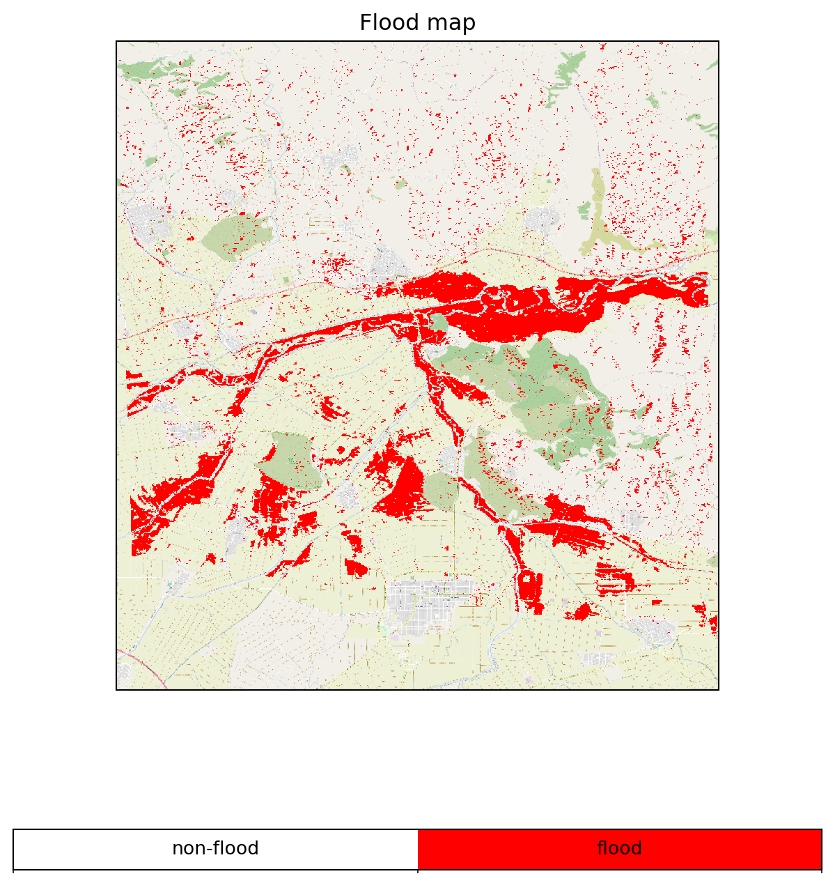
The merged preprocessed datacube can then be used as input for the Bayesian flood mapping function that reduces all these bands to just one in the resulting datacube.
By comparing this figure with the original study (Bauer-Marschallinger et al. 2022), we see that the openEO workflow can perform the same operations. There are, however, some differences with the original flood mapping study. These differences relate to the absence of the low sensitivity masking and post-processing steps of the flood probabilities in the openEO workflow. A priori low sensitivity masking removes observations in which situations arise that cause insensitivity to flood conditions for physical, geometric, or sensor-side reasons. Whereas, post-processing removes e.g. the small patches of supposed flooded pixels scattered throughout the image also known as “speckles”. These speckles produce a more noisy picture in the openEO example.
2.2 Masking of Low Sensitivity Pixels
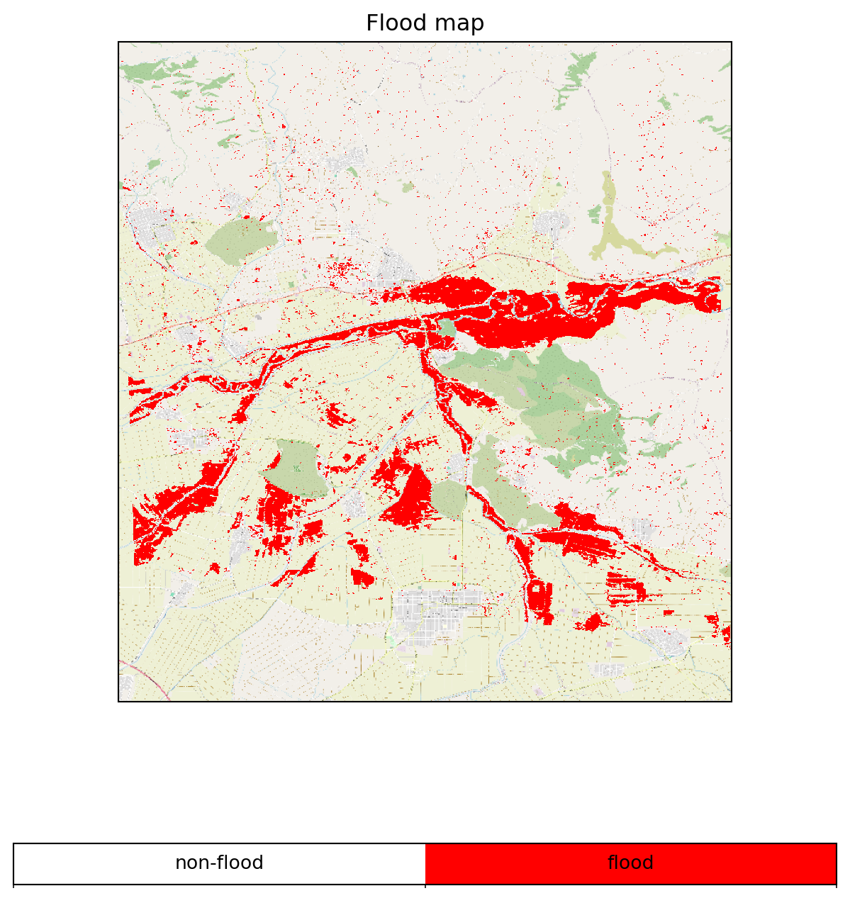
We continue by improving our flood map by filtering out observations that we expect to have low sensitivity to flooding based on a predefined set of criteria.
2.2.1 Masking of Exceeding Incidence Angles
Firstly we mask areas where the incidence angle exceeds the maximum tolerable range of \(27\degree\) to \(48\degree\). These larger than usual incidence angles are a result of the area’s topography as beams reflect from steep slopes.
We remove values that have already low backscatter values during normal conditions and which do not represent water. Examples of such surfaces are highways, airstrips. salt panes, or arid sand and/or bedrock. Identification of such conflicting distribution is done by comparing the expected local land distribution (from the harmonic model) with those from the water distribution, if these cannot be distinguished from each other, the pixel is excluded.
Extreme backscatter values are yet another source of insensitivity to floods. These outliers are not properly represented by the Bayesian model probabilities.
In some cases the posterior distribution is ambiguous as it falls close to a 0.5 probability of flooding (i.e., a coin flip). This happens when the probability distributions for water and land backscattering overlap and/or the measured backscatter values falls exactly in the middle of the two distributions. Hence a cut-off of 0.2 is used to limit the potential of falls positive classifications.
The following steps are designed to further improve the clarity of the floodmaps. These filters do not directly relate to prior knowledge on backscattering, but consists of contextual evidence that supports, or oppose, a flood classification.
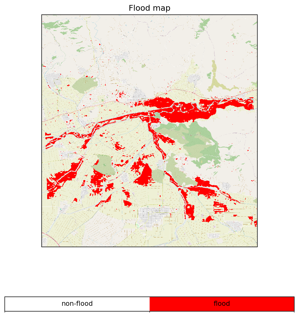
2.3.1 Removal of Speckles
One such filtering approach targets so-called speckles. These speckles are areas of one or a few pixels, and which are likely the result of the diversity of scattering surfaces at a sub-pixel level. In this approach it is argued that small, solitary flood surfaces are unlikely. Hence speckles are removed by applying a smoothing filter which consists of a rolling window median along the x and y-axis simultaneously.
This approach is realized in openEO with the parent function apply_neighborhood() with a window size of 3 by 3 pixels. The child process median is used to average the window’s values.
Bauer-Marschallinger, Bernhard, Senmao Cao, Mark Edwin Tupas, Florian Roth, Claudio Navacchi, Thomas Melzer, Vahid Freeman, and Wolfgang Wagner. 2022. “Satellite-BasedFloodMapping Through BayesianInference from a Sentinel-1 SARDatacube.”Remote Sensing 14 (15): 3673. https://doi.org/10.3390/rs14153673.